Dongjin Seo | Yale University

Designing Photonic Devices with Diffusion Models + Physics: AdjointDiffusion

May 31, 2026

This post is an accessible walkthrough of our paper, “Physics-Guided and Fabrication-Aware Inverse Design of Photonic Devices Using Diffusion Models” (ACS Photonics, 2026). The code is on GitHub. I’ll skip the heavy math and try to give the intuition instead.

The problem: designing a device pixel by pixel

Imagine you want a tiny silicon chip that takes light coming in from one waveguide and splits it into two output ports, maybe sending red light up and blue light down. You get to decide, for every little pixel of a small region, whether it should be silicon or air. A modest design region of $50\times 50$ pixels already gives you $2^{2500}$ possible layouts. You cannot try them all, and most of them do nothing useful.

This is inverse design: instead of guessing a shape and simulating it (“forward”), we specify the performance we want and search for a structure that delivers it.

Two big tools already exist for this, and each has a weakness.

Tool #1: the adjoint method (fast gradients, greedy search)

The adjoint method is the workhorse of photonic inverse design. It answers a remarkably useful question very cheaply:

If I nudge each pixel a little, how much does my device’s performance change?

That is the gradient $\nabla_x \,\mathrm{FoM}(x)$ of the figure-of-merit with respect to every pixel $x$, and the magic is that you get it from just two simulations (one forward, one “adjoint” backward), no matter how many pixels you have. You then take a step uphill:

\[x \leftarrow x + \eta\,\nabla_x \,\mathrm{FoM}(x).\]

This is just gradient ascent on the device. It’s powerful, but it’s local and greedy: it walks uphill from wherever you started and happily gets stuck in a mediocre local optimum. It also has no idea what a “reasonable” device looks like, so it tends to produce blurry, gray, swiss-cheese structures riddled with tiny features that a fab can’t actually manufacture.

Tool #2: diffusion models (a learned sense of “good shapes”)

A diffusion model is the kind of generative model behind modern image generators. The training idea is delightfully physical. Take a clean image (here, a valid device layout) and gradually add noise until it dissolves into pure static. That’s the forward process, and it looks exactly like an ink drop spreading and disappearing into a glass of water:

\[x_t = \sqrt{\bar\alpha_t}\,x_0 + \sqrt{1-\bar\alpha_t}\,\epsilon, \qquad \epsilon \sim \mathcal{N}(0, I).\]

The model then learns to run that movie backwards: starting from random noise and, step by step, removing the noise until a clean, plausible structure emerges. Train it on a library of fabrication-valid devices, and it learns the “grammar” of good layouts: connected waveguides, smooth boundaries, minimum feature sizes. Sampling from it is like un-mixing the ink:

Reverse diffusion: starting from pure noise, the model denoises step by step until a clean, fabricable device layout condenses out, like an ink drop un-mixing from water.

But on its own, a diffusion model only knows what devices look like, not whether they actually work. It has never run a physics simulation. Ask it for “a good splitter” and it gives you something that resembles one, with no guarantee of performance.

The idea: let physics steer the denoising

So we have two halves of the answer:

The diffusion model knows what a fabricable, sensible device looks like.
The adjoint method knows which way is uphill in performance.

AdjointDiffusion combines them. At every step of the reverse diffusion (every time the model removes a bit of noise), we also nudge the structure in the direction the adjoint gradient says will improve performance. Concretely, the usual denoising direction (the model’s score) gets an extra physics term:

\[\underbrace{\nabla_x \log p(x)}_{\text{stay a realistic device}} \;+\; s \cdot \underbrace{\nabla_x \,\mathrm{FoM}(x)}_{\text{improve the physics}}.\]

The first term keeps the design on the manifold of manufacturable structures; the second term pushes it toward better performance. The guidance strength $s$ balances the two. (Readers who know classifier-guided diffusion will recognize the shape: we’ve simply replaced the classifier’s gradient with a physics gradient computed by an FDTD solver.)

At each denoising step, an adjoint (FDTD) simulation computes how to improve the device, and that gradient nudges the generated structure, so efficiency climbs while the design stays fabricable.

The two forces are complementary in a nice way. The physics gradient alone would drag the design off into unfabricable gray mush; the diffusion prior pulls it back to clean, binary, buildable shapes. The diffusion prior alone would settle for something that merely looks right; the physics gradient insists it actually performs. Together they explore the design space far more globally than greedy gradient ascent, finding better optima instead of the first hill they stumble onto.

Plain gradient ascent climbs the nearest hill and plateaus. The generative prior lets AdjointDiffusion keep finding better, still-fabricable optima.

Does it work? Two photonic problems

We tested this on two inverse-design tasks against standard baselines (the Method of Moving Asymptotes, MMA, and plain gradient ascent).

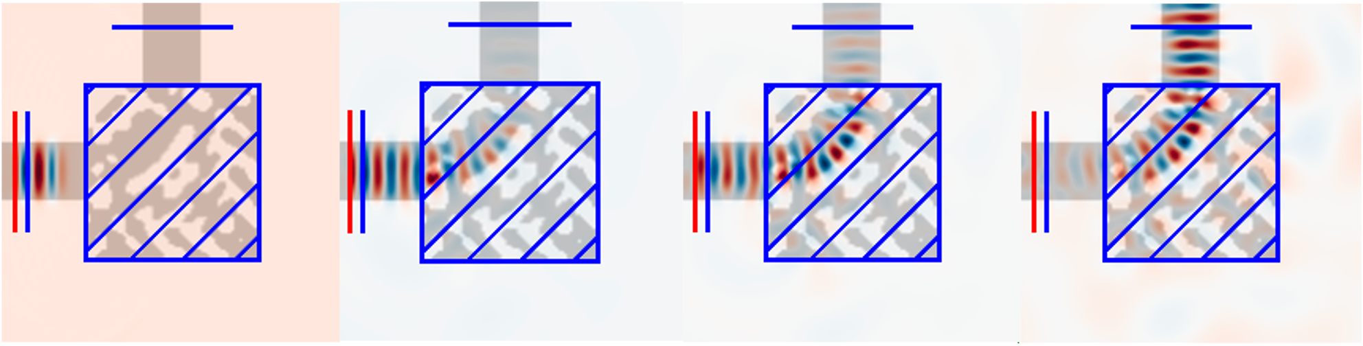
A waveguide / mode device. AdjointDiffusion reaches higher efficiency than the baselines while keeping the structure clean and manufacturable.

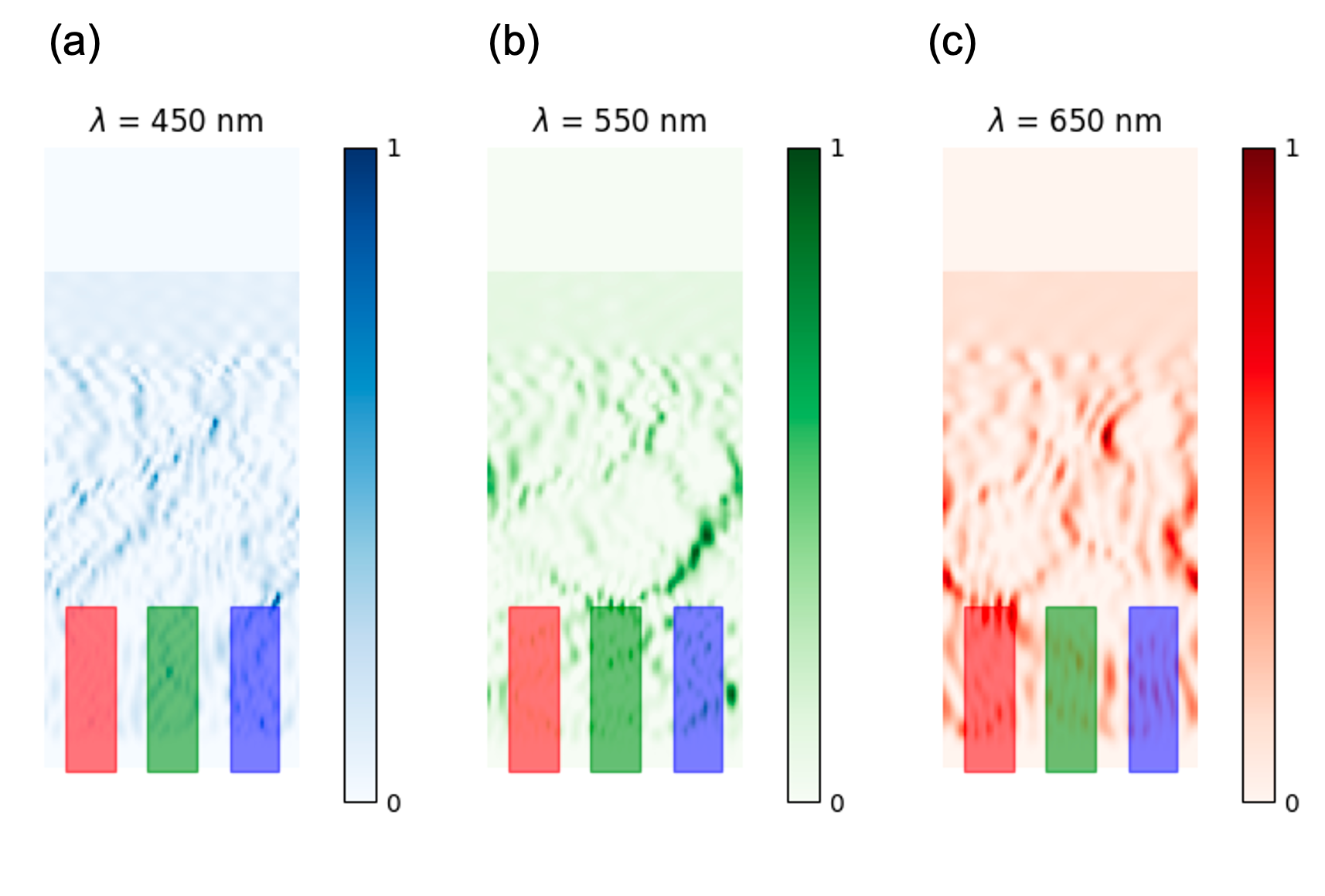
Waveguide optimization results comparing AdjointDiffusion to baselines — Waveguide-device results: AdjointDiffusion vs. baseline optimizers.

A multi-wavelength splitter (“color router”). This is the harder, multi-condition case: the device must do the right thing for several wavelengths at once. We make the diffusion model class-conditional so a single model handles all the target conditions, and the performance converges across wavelengths.

Multi-wavelength color router results — Multi-wavelength splitter ("color router"): one class-conditional model handles multiple target wavelengths.

How it fits together (the pipeline)

If you want to actually run it, the recipe is:

Build a dataset of fabrication-valid structures (dataset_generation.py).
Train a diffusion model on them so it learns the space of buildable devices.
Sample with guidance: during reverse diffusion, call an FDTD solver (Meep) at each step to get the figure-of-merit and its adjoint gradient, and add that gradient to the denoising update.
For multiple targets, condition the model on a class label so one network covers them all.

Plugging in your own physics is meant to be easy: implement a simulation class with compute_fom() and compute_adjoint() methods, and the rest of the machinery carries over.

Takeaways

Inverse design needs both “what’s good” and “what’s buildable.” Adjoint gradients give the first; a generative prior gives the second.
Guided diffusion is a clean way to fuse them: keep the model’s denoising step, add a physics-gradient term, and you get designs that are simultaneously high-performance and fabricable.
It generalizes. Swap in your own simulator and figure-of-merit, and the same framework applies beyond photonics to other physics-constrained design problems.

If you’d like the full details, the paper is here and the code is here.

Citation. D. Seo, S. Um, S. Lee, J. C. Ye, and H. Chung, “Physics-Guided and Fabrication-Aware Inverse Design of Photonic Devices Using Diffusion Models,” ACS Photonics (2026). DOI: 10.1021/acsphotonics.5c00993

← Back to Blog